Excel Tips

Dynamic Named Ranges

Excel functions can be used in a named range if the function returns a cell or range of cells like ADDRESS or OFFSET. The OFFSET function is particularly useful in a named range because it allows the range to vary as the contents change (for example, as data is added or deleted from a column).

In the following example, the header row is not included in the range;

=OFFSET(SheetJ!$A$1,1,0,COUNTA(SheetJ!$A:$A)-1,1) [Don’t forget the dollar signs!]

The first argument [SheetJ!$A$1] sets cell A1 as the anchor for the offset function. The starting and ending cells of the range will be relative to this cell.

The second argument [1] indicates how many rows the start of the range will be from the anchor (so the start of the range will be in row 2).

The third argument [0] indicates how many columns the start of the range will be from the anchor (the starting column of the range will be column A).

The fourth argument [COUNTA(SheetJ!$A:$A)-1] indicates how many rows to include in the range. In this example it will be one less than the number of rows that contain data in column A. Since 6 rows contain data, the range will be 5 rows high. The column used for this doesn’t need to be the same as the column for which the named range is being created.

The fifth argument [1] indicates how many columns wide the range will be.

As data is added or removed from column A, the number of rows in the range will change.

============================================================================

Examples of Functions and Array Formulas

SUMIF can be used for one variable (sales of tables)

=SUMIF(F2:F9,B2,G2:G9) = $ 9,700.

SUMPRODUCT Example (sales of chairs in Minneapolis)

Cell F17: =SUMPRODUCT(($E$2:$E$9=$D17)*($F$2:$F$9=F$13)*($G$2:$G$9)) = $ 1,500.

In this example, If the city in E2 to E9 is equal to D17 (Minneapolis) and if the product in F2 to F9 is equal to F13 (Chair), then add the amounts in G2 to G9 (Total Sale). The answer will be the total sales of chairs in Minneapolis. Each of the ranges (E2:E9, F2:F9 and G2:G9) must have the same number of cells.

Use array formulas [Ctrl-Shift-Enter] for more complex calculations:

Average of table sales in Chicago and Minneapolis;

{=AVERAGE(IF(((E2:E9=A3)+(E2:E9=A5))*(F2:F9=B2),G2:G9))} = $ 2,067.

Count of orders for chairs in Minneapolis;

{=SUM(IF((CityRng=A5)*(ProductRng="Chair"),1,0))} = 2

(CityRng=E2:E9, ProductRng=F2:F9)

============================================================================

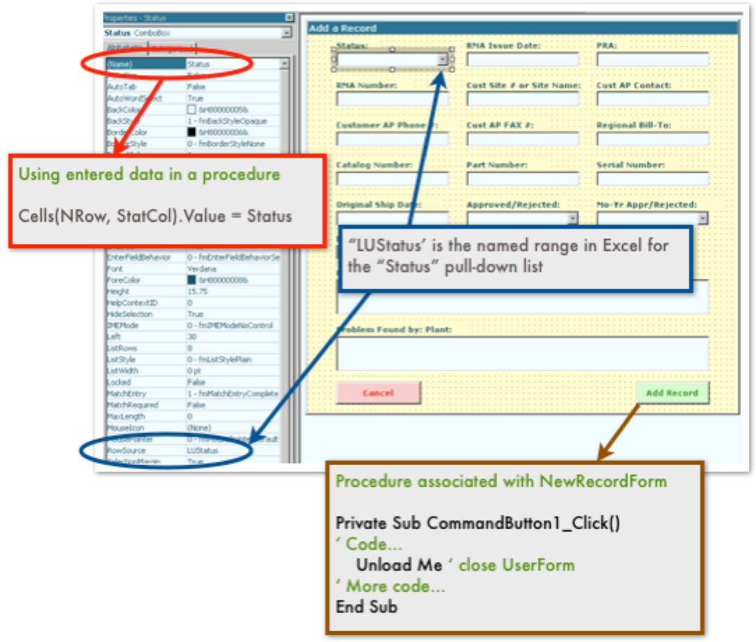
UserForms & ActiveX controls (not available on a Mac)

Procedure to display a UserForm

Sub NewRecord()

NewRecordForm.Show

End Sub

===========================================================================

Excel Tips

To enter the same value or formula in many cells of your spreadsheet, highlight the cells, type the value or the formula and press Ctrl/Enter.

If there isn’t enough room to show all the worksheet tabs, the typical process is to left click on one of the arrows to scroll and find your worksheet. Instead, if you right click on the set of arrows, a list of all your worksheets is shown. If you have more than 15 worksheets, select “More Sheets...” and choose your worksheet.

Sometimes you need a relative reference (B4) sometimes you need an absolute reference ($B$4) and sometimes you need something in between ($B4, B$4). Click on the reference (B4) in the formula bar and press the "F4" key one, two or three times.

To quickly move from a cell to the end of a range of cells, simply double-click on the edge of the selected cell in the direction you want to go.

============================================================================

Favorite Excel Web sites

Beyond Technology http://www.beyondtechnology.com/tips.shtml

Contextures http://www.contextures.com/tiptech.html

John Walkenbach http://www.j-walk.com/ss/excel/index.htm

Jon Peltier-Charting http://peltiertech.com/Excel/Charts/index.html

Mr. Excel Articles http://www.mrexcel.com/articles.shtml

Pearson Software-Topic Index http://www.cpearson.com/excel/topic.htm

============================================================================